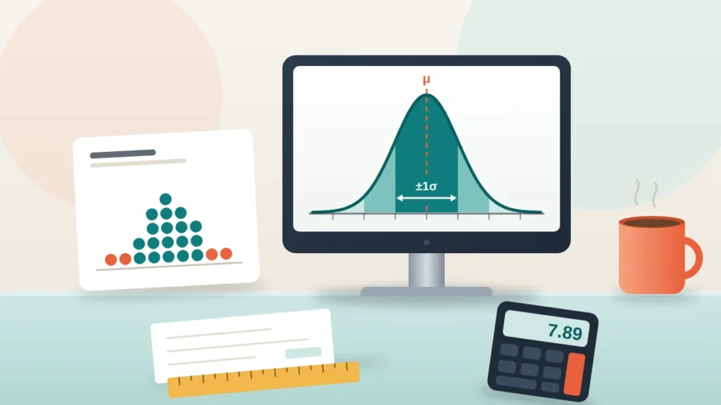
Standard deviation explained in one line: it is the typical distance between each value in a data set and the mean, measured in the same units as the data. To calculate it, find the mean, square each value’s distance from it, average those squares (dividing by n − 1 for a sample), then take the square root.
A small standard deviation means the numbers huddle close to the average. A large one means they are spread out. Two coffee shops can both have an average wait of 5 minutes, but if one has a standard deviation of 0.8 minutes and the other 2.9 minutes, you know which one will make you late for a meeting. This guide works through the calculation by hand, explains the sample vs population question that confuses almost everyone, and shows how the 68–95–99.7 rule and the coefficient of variation turn the number into something useful.
If you have a list of numbers and just want the result, paste it into our standard deviation calculator, which shows every step in a table.
Why the average alone is not enough
Take two coffee shops and record eight wait times at each, in minutes:
- Shop A: 4, 5, 5, 6, 5, 5, 4, 6
- Shop B: 1, 9, 2, 8, 5, 3, 7, 5
Both average exactly 5 minutes. But Shop A never keeps you more than 6 minutes, while Shop B ranges from 1 to 9. The sample standard deviation captures that difference: 0.76 minutes for Shop A and 2.88 minutes for Shop B. Same mean, nearly four times the spread.
That is the whole reason standard deviation exists. The mean tells you where the centre is; the standard deviation tells you how much to trust it as a description of any single value. Manufacturers use it for quality control, investors use it as a measure of risk, teachers use it to see whether a test separated students or bunched them together, and doctors use it to tell whether a child’s height is unusual for their age.
How to calculate standard deviation step by step
Here are eight quiz scores out of 100: 72, 85, 90, 78, 88, 95, 81, 75. The calculation has five steps.
- Find the mean. Add the scores and divide by the count: 664 ÷ 8 = 83.
- Find each deviation. Subtract the mean from every value.
- Square each deviation. This makes every number positive and gives extra weight to values far from the mean.
- Add the squares and divide. The sum is the “sum of squares”. Divide by n for a population or by n − 1 for a sample. The result is the variance.
- Take the square root. That returns you to the original units: points, not points squared.
| Score (x) | Deviation (x − 83) | Squared deviation |
|---|---|---|
| 72 | −11 | 121 |
| 85 | 2 | 4 |
| 90 | 7 | 49 |
| 78 | −5 | 25 |
| 88 | 5 | 25 |
| 95 | 12 | 144 |
| 81 | −2 | 4 |
| 75 | −8 | 64 |
| Sum: 664 | 0 | 436 |
The deviations always add to zero, which is a handy check that you got the mean right. That is also why you cannot just average the deviations: positives and negatives cancel out. Squaring solves that.
Now finish the calculation:
- If these eight students are the whole class (a population): variance = 436 ÷ 8 = 54.5, and σ = √54.5 = 7.38 points.
- If they are a sample from a larger group: variance = 436 ÷ 7 = 62.29, and s = √62.29 = 7.89 points.
Either way, a typical score sits about 7 to 8 points from the class average of 83. The variance calculator stops at step 4 if you need that number, and the sum of squares calculator gives the intermediate total used in regression and ANOVA.
Variance vs standard deviation
Variance is the average squared deviation; standard deviation is its square root. They carry the same information, but in different units. If your data are in dollars, variance is in dollars squared, which nobody can picture. Standard deviation brings you back to dollars.
Statisticians still use variance a lot because it has nicer mathematical properties. Variances of independent quantities add up; standard deviations do not. If two independent measurements each have a standard deviation of 3, their sum has a variance of 9 + 9 = 18 and a standard deviation of √18 = 4.24, not 6. That is the basis of error propagation in lab science and portfolio risk in finance.
Sample vs population: why divide by n − 1
This is the part that confuses students most, and the rule is simpler than it looks.
- Population standard deviation (σ): you have every member of the group you care about. Divide by N.
- Sample standard deviation (s): your data are a subset, and you want to estimate the spread of a bigger group. Divide by n − 1.
The reason for n − 1, called Bessel’s correction, is that a sample’s own mean sits closer to its own values than the true population mean does. Measuring deviations from the sample mean therefore underestimates the real spread a little. Dividing by a slightly smaller number nudges the variance back up to an unbiased estimate. The difference matters for small samples (7.38 vs 7.89 above, a 7% gap with n = 8) and almost vanishes for large ones: with n = 1,000 the two differ by about 0.05%.
In practice, most real data are samples, so s is the default. Spreadsheets reflect this: STDEV.S (or STDEV) in Excel and Google Sheets uses n − 1, and STDEV.P uses N. If you are unsure which to report, use the sample version and say so. The population variance calculator is there for the cases where you genuinely have every value.
The 68–95–99.7 rule
When data follow a roughly bell-shaped (normal) distribution, standard deviation tells you where most values fall:
| Range | Share of values | IQ example (mean 100, SD 15) |
|---|---|---|
| Mean ± 1 SD | About 68% | 85 to 115 |
| Mean ± 2 SD | About 95% | 70 to 130 |
| Mean ± 3 SD | About 99.7% | 55 to 145 |
That is the empirical rule, and it is why “more than two standard deviations from the mean” is a common working definition of unusual. Only about 1 in 20 values lands out there by chance, and only about 3 in 1,000 go beyond three standard deviations. The empirical rule calculator fills in the ranges for any mean and SD, and the NIST/SEMATECH e-Handbook of Statistical Methods covers the normal distribution in depth if you want the theory.
Be careful with skewed data such as incomes, house prices or hospital stays. The rule assumes symmetry. For any distribution at all, Chebyshev’s theorem guarantees only that at least 75% of values lie within 2 SD and at least 88.9% within 3 SD, which is a much weaker promise.
Z-scores: how unusual is one value?
A z-score counts how many standard deviations a value sits from the mean: z = (x − mean) ÷ SD. In the quiz, the student who scored 95 has z = (95 − 83) ÷ 7.89 = 1.52, comfortably above average but not exceptional. The student with 72 has z = −1.39. Pediatricians use the same idea on CDC growth charts, where a child’s height or weight is compared with the reference distribution for their age and sex. Try the z-score calculator to convert any value.
Coefficient of variation: comparing spread across scales
A standard deviation of 5 grams is tiny for a 1 kg bag of flour and enormous for a 50 g jar of saffron. To compare spreads between things measured on different scales, divide the SD by the mean. That ratio is the coefficient of variation (CV), usually shown as a percentage.
- Flour bags: SD 5 g ÷ mean 1,000 g = 0.5%
- Spice jars: SD 2 g ÷ mean 50 g = 4%
The spice line is eight times less consistent, even though its standard deviation is smaller in grams. For the quiz scores, CV = 7.89 ÷ 83 = 9.5%. The coefficient of variation calculator does the division for you. CV only makes sense for data on a ratio scale with a true zero (weights, times, prices), not temperatures in °F or °C.
Standard deviation vs standard error
These two are easy to confuse because both have “standard” in the name and both shrink as data become less noisy. Standard deviation describes how spread out the individual values are. Standard error describes how precisely you have estimated the mean: SE = s ÷ √n. For the quiz, SE = 7.89 ÷ √8 = 2.79 points, which the standard error calculator will confirm.
Collecting more data does not shrink the standard deviation (the students are just as varied), but it does shrink the standard error, because the average of a large sample is more reliable. That is the link to survey design: the sample size guide shows how to choose n so that the standard error, and therefore the margin of error, is as small as you need.
Common mistakes
- Using the population formula on a sample. Most data are samples; divide by n − 1 unless you have everyone.
- Forgetting the square root. If your “standard deviation” is in squared units, you stopped at the variance.
- Applying the 68–95–99.7 rule to skewed data. Check a histogram first.
- Treating SD as an error bar on the mean. Use the standard error or a confidence interval for that.
- Letting one outlier dominate. Because deviations are squared, a single extreme value can inflate the SD a lot. Consider the interquartile range or median absolute deviation for messy data.
- Comparing SDs of things on different scales. Use the coefficient of variation instead.
Frequently asked questions
What does a standard deviation of 0 mean?
Every value is identical. There is no spread at all, so every value equals the mean.
Is a high standard deviation good or bad?
Neither by itself. In manufacturing a low SD usually means consistent quality; in a test designed to rank students, a very low SD may mean the questions failed to separate strong and weak performers.
Can standard deviation be negative?
No. It is the square root of an average of squared numbers, so it is always zero or positive.
Should I use STDEV.S or STDEV.P in Excel?
Use STDEV.S when your data are a sample from a larger group, which is the usual case. Use STDEV.P only when you have every value in the population.
How is standard deviation related to percent error?
Standard deviation measures precision, the scatter of repeated measurements, while percent error measures accuracy against a known value. Our guide to percent error vs percent difference covers the accuracy side.
Once you have computed a standard deviation by hand a couple of times, the number stops being abstract. It is simply the typical gap between a value and the average. Report it next to every mean you publish, pick n − 1 for samples, and use the empirical rule, z-scores and the coefficient of variation to turn that one number into a clear picture of your data.